-
Notifications
You must be signed in to change notification settings - Fork 8
Extending the first simulation
The example from First Simulation created a world and added 800 nodes within an area of size 25x25 that sent one message at boot time, and then deactivate themselves if they do not receive a message for 5 rounds. To consider a larger scenario we will expand the size of the simulated world, and also put more processors into the world. Hence, change your configuration file as follows:
  prepare_world edge_model=simple comm_model=disk_graph range=1
  rect_world width=50 height=50 count=5000 processors=helloworld
  simulation max_iterations=10
  connectivity
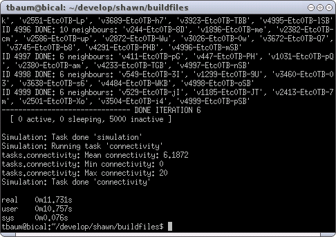
The number of processors increased to 5000, and therefore the size of the world grows to a 50x50 field. In addition, a new task is executed after the simulation finished. The task named connectivity is also part of the examples application, and shows the average number of neighbors of the nodes (as well as the minimum and maximum value). However, running this example by also using the time command in Linux that shows how long processes ran ends up as shown in Figure XXX.

The execution took approximately 12 seconds, and should have run straight through, but with a noticeable delay after running the task connectivity. Now we run the simulation again, but we use an alternative edge model. The configuration looks as follows (note the edge model list instead of simple):
  prepare_world edge_model=list comm_model=disk_graph range=1
  rect_world width=50 height=50 count=5000 processors=helloworld
  simulation max_iterations=10
  connectivity
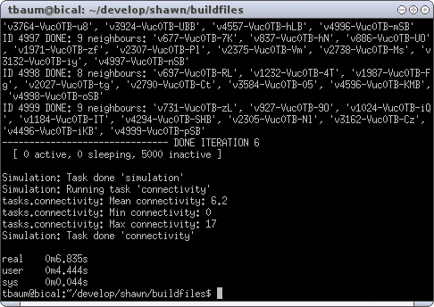
The result is shown in Figure XXX.

The execution took approximately 7 seconds, and thus was 4 seconds
faster than the one with the simple edge model. As you may have
noticed, the output (ID 'X' GOT HELLO FROM 'Y') of the
simple one was slightly slower than the list one, but
there was a delay after starting the connectivity
task. Contrary, the task rect_world delayed when using the
list model, but everything else executed straight through.
The differences can be explained as follows. The simple edge model should particularly used for small topologies with approximately a few thousand nodes (depending on the applications attached to the nodes). On 'each' transmitted message, 'all' nodes are checked for potential receivers. Then, the task connectivity delayed because for 'each' node in the topology, 'all' nodes were checked for potential neighbors (and counted, if so). In contrast, the list model pre-calculates the neighborhood of each node. Thus, the task rect_world is delayed because for 'each' node in the topology, 'all' other nodes were checked 'once' for being potential neighbors. The neighbors are stored in a list, and used for message transmission (when a node sends a message, the receivers are already known) and neighborhood iteration (just running through the known list). Thus, the execution with the list model was faster than the one using the simple edge model.
When the task rect_world is used in the beginning of a simulation, the topology is created randomly. Consequently, if you run two simulations one after the other, both runs will probably produce different results. If you want to rerun simulations, you must use the same random seed for both simulations. Shawn therefore provides the simulation task random_seed that can be used for storing and loading the used seed.
Hence, if you run a simulation, add
random_seed action=create filename=file_containing_the_seed
as the first line in your configuration file. Then, the used seed can be found in the file file_containing_the_seed. When you want to rerun a simulation, write
random_seed action=load filename=file_containing_the_seed
instead. Alternatively, the random seed can also be set directly with
random_seed action=set seed=123456789
We will use this task in the ongoing examples to point out the purpose of this task.
So far you have run several simulations, from a few hundred nodes to 5000. In addition, you have tried different edge models (simple and list), and you can reproduce simulation results. Now let us have a look at the Transmission Model. If not given, the standard transmission model is the reliable one. That is, each sent message which can be received by a node is definitely received.
In general, it is possible to use multiple transmission models. Each model owns therefore the state chainable. If set to true, another model can be added. If not, the model has to be an end point (that is, it is not allowed to add further models). Message sending then looks as follows.
Message -> ChainTransModel1 -> ChainTransModel2 -> EndTransModel
If a message is sent, it is handed over from model to model, beginning with the first in the configuration file. A model is also able to drop messages, so that the message does not reach each model at any time.
However, look at the following example:
  random_seed action=create filename=.rseed

  prepare_world edge_model=list comm_model=disk_graph \
      transm_model=stats_chain \
      range=1
  chain_transm_model name=reliable

  rect_world width=50 height=50 count=5000 processors=helloworld
  simulation max_iterations=10

  connectivity
  dump_transmission_stats
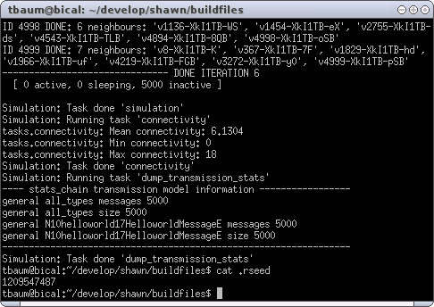
First, the seed task has been added that stores the used seed into the file .rseed. Then, prepare_world got an extra parameter transm_model which is set to stats_chain. This model is chainable (as implied by the name) and collects statistics of the overall sent messages. In the consequence that only information is collected, but no messages are sent, the task chain_transm_model in the next line adds the reliable transmission model which transmits 'each' message without delay or loss. The next lines are the same as for the previous simulations, except for the last one. dump_transmission_stats is a simulation task that collects the information from chain_transm_model and prints it out. The result of running Shawn is shown in Figure XXX.

After the already known output of the connectivity task there is the result of dump_ transmission_stats. It shows that 5000 messages were sent (obvious when 5000 nodes send exactly one message at boot time), and that the type of the messages was HelloWorldMessage. The output format may differ if you use a different compiler (here: g++ (GCC) 4.2.3), because the return value of name() from typeinfo is not standardized and depends on the compiler. However, after the simulation finished, the used seed is printed to the terminal (here: 1209547487). Note the number of neighbors of node 4998 (6) as well as the average connectivity (6.1304).
Next, another transmission model is added to the chain. Look at the updated configuration file:
  random_seed action=load filename=.rseed

  prepare_world edge_model=list comm_model=disk_graph \
    transm_model=stats_chain \
    range=1
  chain_transm_model name=random_drop_chain probability=0.1
  chain_transm_model name=reliable

  rect_world width=50 height=50 count=5000 processors=helloworld
  simulation max_iterations=10

  connectivity
  dump_transmission_stats
There happened two changes. First, the action of simulation task random_seed changed to load (to use the previous seed of 1209547487). Second, task chain_transm_model is called one more time. It adds transmission model random_drop_chain that drops messages with a given probability (here, set to 10%). Now, the transmission model chain looks as follows.
Message -> StatsChain -> RandomDropChain -> Reliable
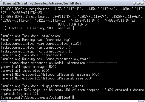
If a message is sent, it is first handed to StatsChain that stores count and type of the message. Then, the message is handed over to the RandomDropChain that drops the message with a probability of 0.1. If not dropped, the message is given to the Reliable model that delivers it to the receiver. Have a look at the result shown in Figure XXX.

As a result of using the same seed as before, the same scenario as before was simulated. This is indicated by the same average connectivity of 6.1304. But have a look at the neighborhood of node 4998. Now, it shows only 4 neighbors (instead of the 6 before). This is caused by the additional message loss. The last line in the screenshot shows that 481 messages were dropped, and therein contained the two missing HelloWorld messages directed to node 4998.